TFGA

TensorFlow-based framework for Geometric Algebra

About me

Robin Kahlow

Machine-Learning and Software Engineer with Cambrian working on Home Visualization
Areas: Machine Learning, Augmented Reality, Computer Vision

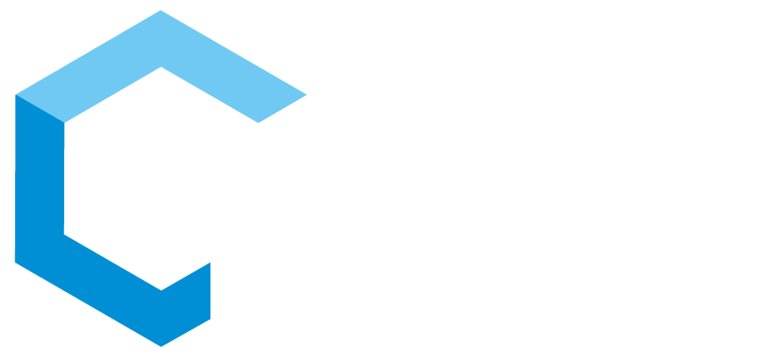
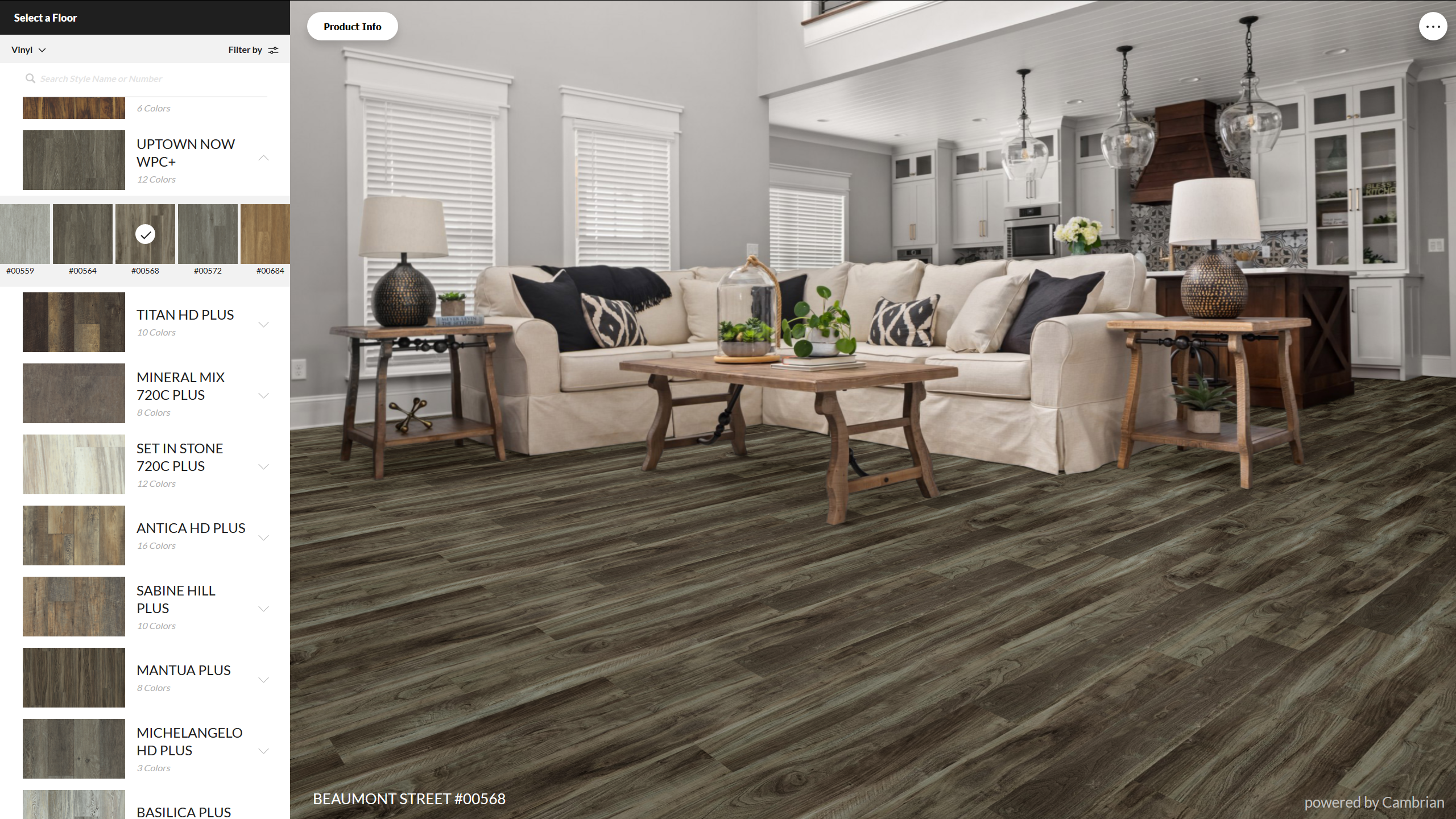FLOORVANA+ (Shaw Floors)

Masked plane finder

Task: Find masked planes in image
Solution: Use neural networks that takes image and outputs masked planes
Problems
- How to parameterize planes in neural networks?
- What is a good neural network architecture for geometric problems?
Possible answer: Geometric Algebra

Structure

TensorFlow
Neural Networks
Geometric Algebra
Geometric Algebra in TensorFlow
Geometric Algebra Neural Networks
Applications
1. LieNet
2. Joint Transform Estimation
3. Lattice QFT
Conclusion and Future work

1. TensorFlow

Machine-learning framework for building models
Runs on many devices (CPUs, GPUs, TPUs)
Supports distributed computing
Easy to use (since version 2)
Automatic differentiation
Widely used, a lot of documentation
Mainly for Python

Tensors in TF - Multidimensional arrays

List of numbers

$[1, 7, 5]$


                            tf.constant([1, 7, 5],
                                dtype=tf.float32)

Identity matrix

$\delta_{ij}$


                            tf.eye(num_dims)

3D ones

$\mathbb{1}_{ijk}$


                            tf.ones([size_i, size_j, size_k])

Operations on Tensors

Addition

$A_{ijk} + B_{ijk}$


                            a + b

Elementwise sine

$sin(A_{ij})$


                            tf.sin(a)

Matrix multiplication

$A_{ij} B_{jk}$


                            tf.matmul(a, b)

Einstein-ish notation

$\sum_{k} A_{ijk} \cdot B_{ikl} = A_{ijk} B_{ikl} = C_{ijl}$


                        c = tf.einsum("ijk,ikl->ijl", a, b)

Keep $i$, $j$, $l$ (appear on $C_{ijl})$
Sum over $k$ (doesn't appear on $C_{ijl}$)

Automatic differentiation

\[\begin{aligned} y(x) & = x^2 & \frac{\delta y}{\delta x}(x) & = 2x \\ y(3) & = 9 & \frac{\delta y}{\delta x}(3) & = 6 \end{aligned} \]


                        x = tf.constant(3)
                        with tf.GradientTape() as tape:
                            y = x ** 2 # 9

                        print(tape.gradient(y, x)) # 6

2. Neural Networks

Input $x_i$, output $y_j$, weight matrix $W_{ij}$
Supervised learning: adjust $W$ to minimize error on dataset

\[\begin{aligned} y_{j} & = W_{ij} x_{i} & \mbox{(Matrix multiplication)}\\ y_{j} & = W_{ij} x_{i} + c_{j} & \mbox{(+ Bias)}\\ y_{bj} & = W_{ij} x_{bi} + c_{j} & \mbox{(+ Batch dimension)}\\ y_{bj} & = f(W_{ij} x_{bi} + c_{j}) & \mbox{(+ Activation function)} \end{aligned} \]

$z_{bj} = W_{ij} x_{bi} + c_{j}$

$y_{bj} = f(z_{bj}) = relu(z_{bj})$


                            def dense(x, w, c):
                                z = tf.matmul(w, x) + c
                                # or z = tf.einsum("ij,bi->bj", w, x) + c

                                y = tf.nn.relu(z)
                                return y
                            
                            # x has shape [batch, in_units]
                            w = tf.Variable(tf.random.normal([x.shape[1], 10]))
                            c = tf.Variable(tf.zeros([10]))

                            with tf.GradientTape() as tape:
                                y = dense(x, w, c)
                            dy_dw = tape.gradient(y, w)

Keras - Layers as objects


                        # Layer contains variables.
                        # Returns relu(Wx + c) when called.
                        dense_layer = tf.keras.layers.Dense(
                            units=10, activation="relu"
                        )
                        
                        # x has shape [batch, in_units]
                        y = dense_layer(x)

                        # Can reuse layer without creating new variables
                        v = dense_layer(u)

Point-cloud Classification


                        network = Sequential([
                            Dense(units=64, activation="relu"),
                            Dense(units=64, activation="relu"),
                            Dense(units=40, activation="softmax")
                        ])
                        # loss: term to be minimized
                        network.compile(loss="categorical_crossentropy",
                                        optimizer="Adam")

                        # inputs: [num_samples, 3*2048] (2048 3d points)
                        # outputs: [num_samples, 40] (40 classes)
                        model.fit(train_inputs, train_outputs,
                                  epochs=10, validation_split=0.1)

                        predictions = model.predict(test_inputs)

3. Geometric Algebra

Basis vectors $\{e_x, e_y\}$, Vector $v = v_x e_x + v_y e_y$

Parallel vectors: $e_{x}e_{x} = 1$

Orthogonal vectors anti-commute: $e_{x}e_{y} = -e_{y}e_{x}$

\[\begin{aligned} a b = & (a_x e_x + a_y e_y) & & (b_x e_x + b_y e_y) & = \\ & a_x b_x + a_y b_y & + & (a_x b_y - a_y b_x) e_x e_y & = \\ & a \cdot b & + & a \wedge b & \\ \end{aligned} \]

Inner Product Exterior Product

Summary

Basis vectors: $\{e_0, ..., e_n\}$
Inner product: $e_i \cdot e_j = \begin{cases} -1 / 0 / 1, & i = j \\ 0, & i \neq j \end{cases}$
Exterior product: $e_i \wedge e_j = \begin{cases} 0, & i = j \\ e_{ij}, & i \neq j \end{cases}$
Geometric product: $a b = a \cdot b + a \wedge b$
Exterior product anti-commutes: $e_{ij} = -e_{ji}$

Complex numbers / 2D rotation

$e_x^2 = e_y^2 = 1 \implies e_{xy}^2 = -1$
Quaternions / 3D rotation

$e_x^2 = e_y^2 = e_z^2 = 1 \implies e_{xy}^2 = e_{yz}^2 = e_{xz}^2 = -1$
Spacetime algebra (Quantum Electrodynamics, Gravity (GTG))

$e_t^2 = 1, e_x^2 = e_y^2 = e_z^2 = -1$
Projective Geometric Algebra (Translations, Rotations, Reflections, Euclidean motion)

$e_0^2 = 0, e_x^2 = e_y^2 = e_z^2 = 1$

4. GA in TensorFlow

Geometric product: multiplication table

For $e_1^2 = e_2^2 = 1$

1	e₁	e₂	e₁₂
e₁	1	e₁₂	e₂
e₂	-e₁₂	1	-e₁
e₁₂	-e₂	e₁	-1

Example: $table[e_1, e_{12}] = e_2$

or with blade-indices (Scalar: 0, $e_1$: 1, $e_2$: 2, $e_{12}$: 3): $table[1, 3] = 2$

Can be precomputed

Multivectors: basis blade coefficients as 1-Tensor

Eg.: a = $1 + 2 e_x + 3 e_y + 4 e_{xy} \rightarrow [1, 2, 3, 4] = a_i$

Dense representation of mult. table as 3-tensor

$C_{ijk}$

$a b = y \rightarrow a_i b_j C_{ijk} = y_k$


                        a = tf.constant([1, 2, 3, 4]) # shape [4]
                        b = tf.constant([3, 9, 7, 5]) # shape [4]
                        # c is precomputed and has shape [4, 4, 4]
                        y = tf.einsum("i,j,ijk->k", a, b, c) # y shape [4]

Benchmarks

Geometric product

Benchmarks

Addition

Reminder: Automatic differentiation

$y = a b, \frac{\delta y(a, b)}{\delta a}$


                        a = tf.constant([1, 2, 3, 4]) # shape [4]
                        b = tf.constant([3, 9, 7, 5]) # shape [4]
                        with tf.GradientTape() as tape:
                            # c is precomputed and has shape [4, 4, 4]
                            y = tf.einsum("i,j,ijk->k", a, b, c)

                        print(tape.gradient(y, a)) # = d/da_i sum(y_j), has shape [4]
                        print(tape.jacobian(y, a)) # = d/da_i y_j, shape [4, 4]

TFGA - Tensor API


                        ga = tfga.GeometricAlgebra([1, 1, 1])

                        # Create geometric algebra tf.Tensor for vector blades
                        # (ie. e_0 + e_1 + e_2).
                        # Result: tf.Tensor [0, 1, 1, 1, 0, 0, 0, 0]
                        vector = ga.from_tensor_with_kind(
                            tf.ones(3), kind="vector"
                        )
                        # 5 + 5 e_01 + 5 e_02 + 5 e_12
                        # tf.Tensor [5, 0, 0, 0, 5, 5, 5, 0]
                        quaternion = ga.from_tensor_with_kind(
                            tf.fill(dims=4, value=5),
                            kind="even"
                        )
                        ga.print(ga.geom_prod(vector, quaternion))

TFGA - Tensor API


                        # Grade reversal ~(5 + 5 e_01 + 5 e_02 + 5 e_12)
                        # = 5 + 5 e_10 + 5 e_20 + 5 e_21
                        # = 5 - 5 e_01 - 5 e_02 - 5 e_12
                        ga.print(ga.reversion(quaternion))

                        # tf.Tensor of shape [1]: -5
                        # (ie. reversed sign of e_01 component)
                        ga.print(ga.select_blades(quaternion, "10"))

                        # tf.Tensor of shape [8] with only e_01
                        # component equal to 5
                        ga.print(ga.keep_blades(quaternion, "10"))

                        # Exterior product e_01 ^ e_2 = e_012.
                        ga.print(ga.ext_prod(ga.e01, ga.e2))

TFGA - MultiVector API


                        ga = tfga.GeometricAlgebra([1, 1, 1])
                        a = ga.from_tensor(...)
                        b = ga.from_tensor(...)

                        # Wraps tf.Tensors in tfga's MultiVector class which
                        # provides operator overrides etc.
                        mv_a = ga(a)
                        mv_b = ga(b)
                        
                        # Reversion ((~mv_a).tensor equivalent to ga.reversion(a))
                        print(~mv_a)
                        # Geometric / inner / exterior product
                        print(mv_a * mv_b, mv_a | mv_b, mv_a ^ mv_b)
                        # Get back tf.Tensor from the multivector
                        print(mv_a.tensor)

Tensor vs MultiVector API

Tensors: easy TensorFlow interop
MultiVector: less verbose, no overhead

5. GA Neural Nets

Standard Dense Layer: $y_{bj} = f(W_{ij} x_{bi} + c_j)$

$W_{ij} \in \mathbb{R}^{MN}, c_j \in \mathbb{R}^N$


                        dense_layer = Dense(
                            units=64, activation="relu"
                        )

GA Dense Layer: make parameters multivector-valued

$W_{ij} \in \mathbb{Cl}_{(p,q,r)}^{MN}, c_j \in \mathbb{Cl}_{(p,q,r)}^N$


                            # Create algebra with 3 basis vectors squaring to 1
                            ga = tfga.GeometricAlgebra([1, 1, 1])

                            # 1, e01, e02, e12 indices: [0, 4, 5, 6]
                            even_indices = ga.get_kind_blade_indices("even")
                            # e0, e1, e2, e012 indices: [1, 2, 3, 7]
                            odd_indices = ga.get_kind_blade_indices("odd")
                            
                            ga_dense_layer = tfga.layers.GeometricProductDense(
                                algebra=ga,
                                units=64, activation="relu",
                                kernel_blade_indices=even_indices,
                                bias_blade_indices=odd_indices
                            )

Choices

Activation function $f$: elementwise or acting on multivector (eg. $e^{a e_{12}} = cos(a) + e_{12} sin(a)$)?
Geometric product $W_{ij} x_i$ or Sandwich product $W_{ij} x_i \widetilde{W}_{ij}$
Matrix mult $W_{ij} x_i$ or elementwise mult $W_{i} x_i$
Add bias $c_{j}$?
Algebra / signature
Subalgebra for $W_{ij}$ and $c_{j}$

No activation, sandwich product, elementwise multiplication, no bias, quaternion weights

$y_i^{(1)} = W_{i} x_i \widetilde{W}_{i}$

Two layers

$y_i^{(2)} = U_{i} y_i^{(1)} \widetilde{U}_{i} = U_{i} W_{i} x_i \widetilde{W}_{i} \widetilde{U}_{i}$

Composition of transforms

Multi-layer reduces to one layer

Log input, Exp on final output, ReLU activation, geometric product, matrix multiplication, bias, quaternion weights

$x_i^{(1)} = log(x_i^{(0)})$

$x_j^{(n+1)} = relu(W_{ij}^{(n)} x_i^{(n)} + c_j^{(n)})$

$y_j = e^{W_{ij}^{(N-1)} x_i^{(N-1)} + c_j^{(N-1)}}$

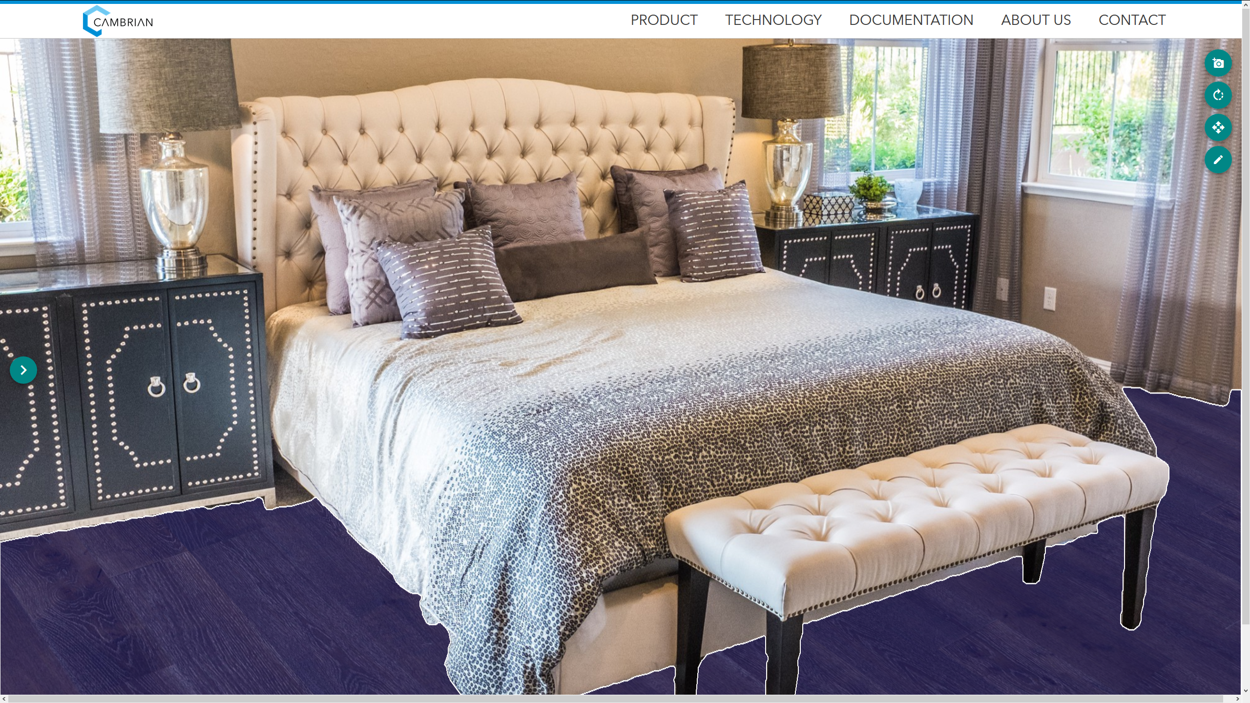
$log$ goes from Lie group to algebra

$exp$ goes from Lie algebra to group

6. GA-NN Applications

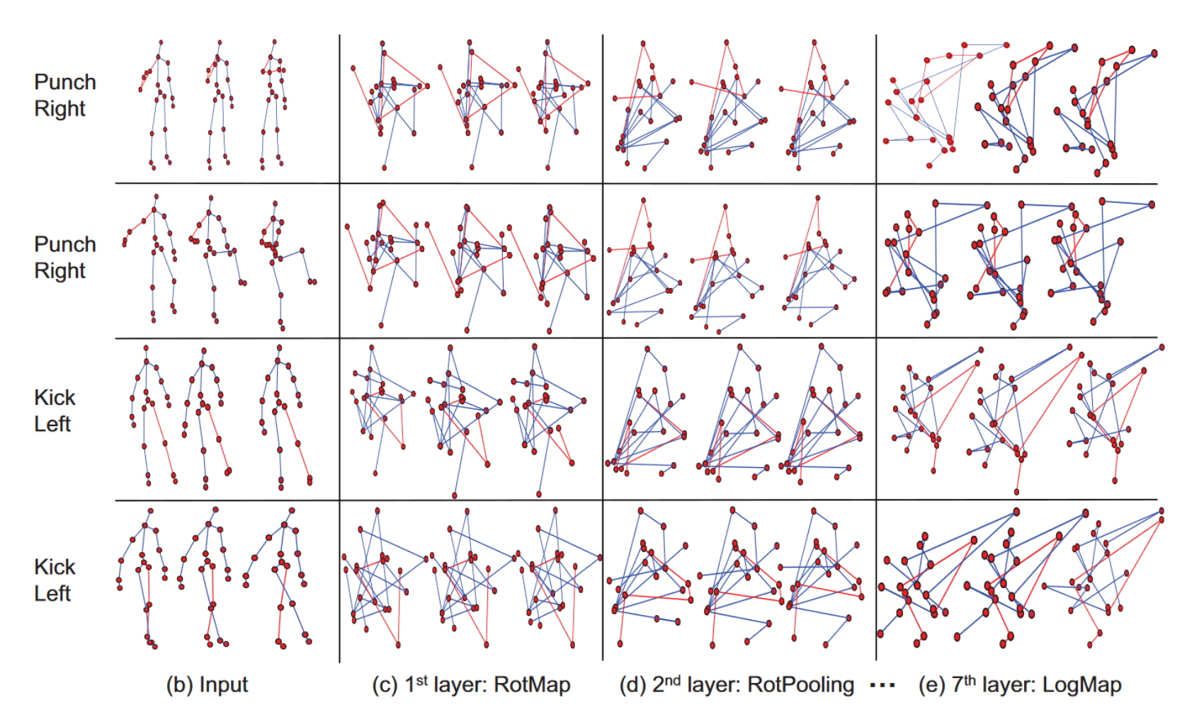
6.1 LieNet

Deep Learning on Lie Groups for Skeleton-based Action Recognition

Implementation in TFGA by Hugo Hadfield


                        ga = GeometricAlgebra([1, 1, 1])

                        model = Sequential([
                            TensorToGeometric(ga, blade_indices=[6, 5, 4, 0]),
                            RotMap(ga, use_bias=False), 
                            LogMap(ga),
                            Flatten(),
                            ReLU(),
                            Dense(units=20),
                            Softmax(axis=-1)
                        ])

Train model on dataset (Pose-sequence $\rightarrow$ Action)


                        model.compile(
                            optimizer="Adam", 
                            loss="sparse_categorical_crossentropy",
                            metrics=["sparse_categorical_accuracy"]
                        )

                        model.fit(
                            x=inputs_train, y=labels_train, 
                            validation_data=(inputs_test, labels_test),
                            epochs=100
                        )

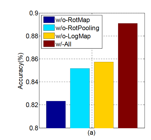
Results

Relatively easy and quick to implement using TFGA
Accuracy verified
But: outperformed by simple Dense ReLU NN (~90% accuracy)

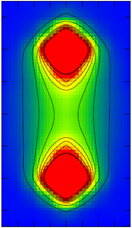
6.2 Joint Transform Estimation

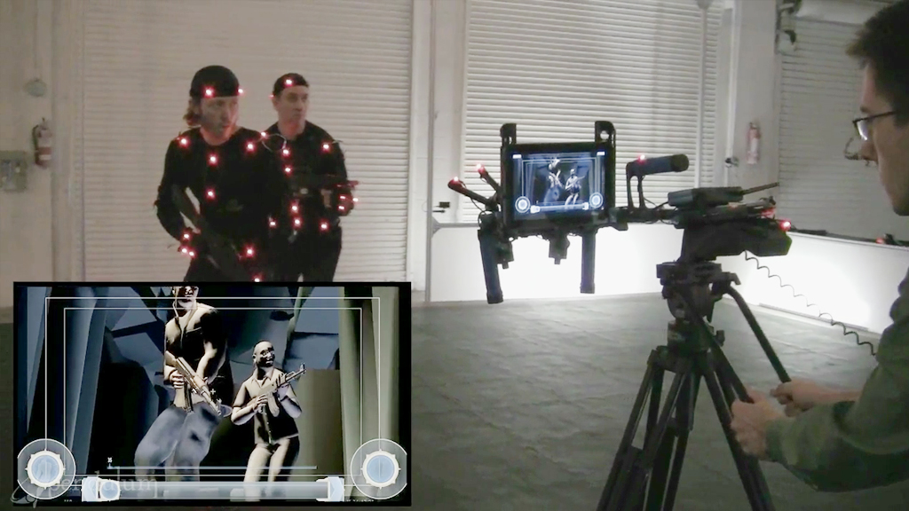
https://www.phasespace.com/applications/3dcharactercreation/

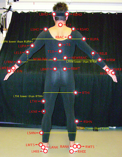
Data: extract frames from CMU MoCap dataset
Each joint has position and rotation
Representation: Motors in 3D-PGA
Task: given 6 joints' transforms, predict other 31 joints' transforms
Compare Dense GA NN vs Standard Dense NN

Data and Ganja.js visualization: Steven De Keninck

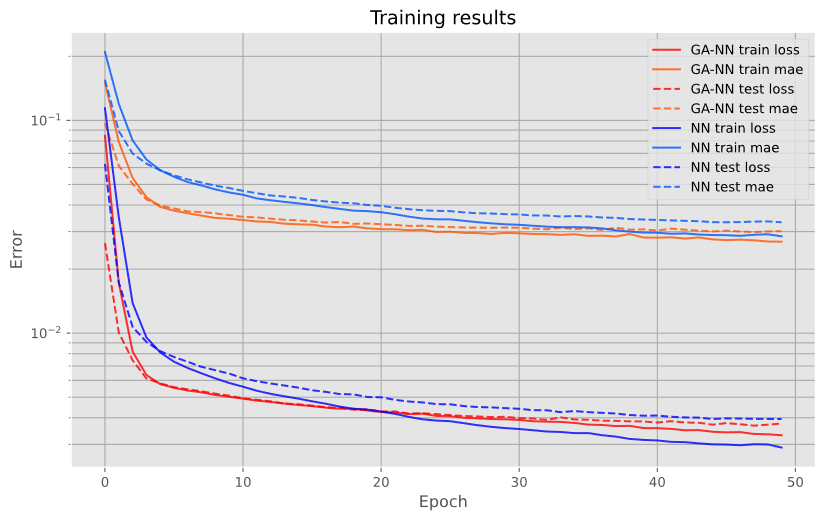
Results

GA NN converges quicker, but might just be due to initialization
Both converge to same test error

6.3 Lattice QFT

\[\begin{aligned} \mathcal{L}_{QED}(X) = & \langle \hbar (\nabla \psi(X)) \gamma_2 \gamma_1 \gamma_3 \widetilde{\psi}(X) - \\ & e A(X) \psi(X) \gamma_0 \widetilde{\psi}(X) - \\ & m \psi(X) \widetilde{\psi}(X) \rangle_0 \end{aligned} \]

Action $S = \int_{\mathcal{X}} \mathcal{L}(X) dX$

Many cells, many parallel calculations, perfect for TensorFlow
TensorFlow Probability provides MCMC samplers (or variational inference) needed for lattice QFT

$m \psi(X) \widetilde{\psi}(X)$


                        sta = tfga.GeometricAlgebra([1, -1, -1, -1])
                        
                        def get_mass_term(psi, electron_mass):
                            return (electron_mass *
                                sta.geom_prod(psi, sta.reversion(psi)
                            )

$e A(X) \psi(X) \gamma_0 \widetilde{\psi}(X)$


                        def get_interaction_term(psi, a, electron_charge):
                            return sta.geom_prod(
                                electron_charge * a,
                                sta.geom_prod(
                                    psi,
                                    sta.geom_prod(sta.e0, sta.reversion(psi))
                                )
                            )

$\hbar (\nabla \psi(X)) \gamma_2 \gamma_1 \gamma_3 \widetilde{\psi}(X)$


                        def get_momentum_term(psi, spacing, hbar):
                            dt_psi = finite_differences(psi, axis=0, spacing=spacing)
                            dx_psi = finite_differences(psi, axis=1, spacing=spacing)
                            dy_psi = finite_differences(psi, axis=2, spacing=spacing)
                            dz_psi = finite_differences(psi, axis=3, spacing=spacing)
                            d_psi = dt_psi + dx_psi + dy_psi + dz_psi

                            return sta.geom_prod(
                                hbar * d_psi,
                                sta.geom_prod(sta.e213, sta.reversion(psi))
                            )

Sum cells' $\mathcal{L}$ to get Action $S$


                        def get_action(psi, a, electron_charge):
                            mass_term = get_mass_term(psi=psi,
                                electron_mass=electron_mass)
                            int_term = get_interaction_term(psi=psi,
                                a=a, electron_charge=electron_charge)
                            mom_term = get_momentum_term(psi=psi,
                                spacing=spacing, hbar=hbar)
                        
                            # Sum terms and get scalar part
                            lagrangians = (mom_term - mass_term - int_term)[..., 0]
                        
                            return tf.reduce_sum(lagrangians)

7. Conclusion and Future work

Conclusion

Fast implementation of GA on GPUs
Easy to implement GA NNs with TFGA
Also usable for other high-dimensional problems

Future work

Exploit sparsity in GPU-friendly way (AST-rewrite / metaprogramming?)
Custom CUDA kernels for GA operations
Improve API consistency (eg. blade arguments)
More layers, more operations, ...
Explore and implement more applications

Questions

TFGA on GitHub

Bivector Discord

My email: tora@warlock.ai